Sensitivity (updated March 2023)
This page provides information necessary to plan MODS spectroscopic and imaging observations. The grating zeropoints and signal-to-noise tracks were updated in January 2023, based on spectrophotometric standards observed in September and October 2022. The imaging zeropoints were updated for MODS1 and added for MODS2, based on data taken on February 10, 2023 UT. (A spectrophotometric standard star was also observed on Feb 10, 2023 UT, and the spectroscopic zeropoints measured from it and are about <0.05 dex lower than the values reported here.)
Although the sensitivities of MODS1 and MODS2 were nearly identical at commissioning, they, or rather the combined instrument+telescope throughput which is what is measured by the spectrophotometric standards, have changed over time. By the time the first MODS2 observations were made, a difference of approximately a factor of ~2 was noted between the counts (factor ~1.4 in electrons) in MODS1 and MODS2 red channel images, both in the object and also the background (TBC whether the factor is exactly the same for both). The discrepancy has increased and the relative photon flux ratio of MODS2 with respect to MODS1 is currently about a factor of 2 (factor ~3 in counts). This difference affects all grating and imaging modes (dual and direct; we have not compared the prism modes). If it affects both the signal and the sky background similarly, then, assuming that the dominant source of noise is the sky background, to achieve the same SNR with MODS1 as with MODS2 would require an exposure that is two times as long.
The table of MODS1 & MODS2 grating zeropoints had last been updated on April 23, 2020 (based on data from 2019-2020). In comparison to these, the September-October 2022 zeropoints are approximately 0.09-0.1 dex worse for MODS1 and about 0.03-0.04 dex better for MODS2.
The SNR tracks below assume these updated zeropoints. The calculation of these SNR tracks assumes a Gaussian PSF to account for slit losses and to determine the contribution from the sky. The extraction window is assumed to cover Nrows = 2.4 * FWHM rows and contains 99.5% of the light.
Spectroscopic Mode
The predicted counts per angstrom at a given wavelength, airmass and exposure time, may be calculated using the formula,
log Sλ = log Sλ ,0 + log Fλ + log texp – 0.4 Kλ X
where:
log Sλ = log counts in ADU Å-1 at wavelength λ
log Sλ ,0 = Spectroscopic zero point in ADU Å-1at wavelength, see tables below.
Fλ = flux in units of erg/sec/cm2/Å
texp = exposure time in seconds
Kλ = estimated extinction coefficient at wavelength λ
X = airmass at the time of the observation
To convert AB magnitudes to Fλ:
log Fλ = -0.9608 – 0.4 AB – 2 log λ
where: AB = Spectral AB magnitude and λ is the wavelength in Angstroms.
The spectroscopic zero points at selected wavelengths for the MODS red and blue grating and prism modes are listed in the tables 1 and 2 below. For a given source flux (Fλ), exposure time and airmass, these allow a 10-20% prediction of counts per angstrom, Sλ, which can be converted to counts per pixel when multiplied by the spectral pixel size in Å. The effect of atmospheric extinction is factored in by selecting a nominal airmass for the observation and applying an appropriate model for the atmospheric extinction (see below). A caveat — predictions based on these zero points should be considered as for the best-case scenario, as there are various observational factors that can degrade the sensitivity achieved: slit losses, which depend on seeing among other factors; changes in sky brightness with time, telescope pointing or moon phase and distance from target; changes in transparency; and changes in the reflectivities of the telescope or instrument optics, are some examples.
Grating Mode
The efficiencies for the grating spectroscopic modes, based on MODS1+SX and MODS2+DX data from September 25, 2022 UT. These efficiencies are for MODS1 plus the LBT SX primary and secondary mirrors and MODS2 plus the LBT DX primary and secondary mirrors and are exclusive of the atmosphere (I use the diameters of the primaries and their central obscurations, but assume perfect reflectivities, and I assume airmass=0). The efficiency of MODS1+SX has decreased by approximately a factor of 2 since the time of commissioning when efficiencies were similar to those of MODS2. The decrease is wavelength-dependent although not monotonic across both channels or even in one channel. Also, the red-only efficiencies of both MODS1 and MODS2 have decreased with respect to the dual modes above 6000 or 7000 angstroms, possibly due to some degradation of the Ag coatings on the flat mirrors in the red channel. The upturn in red-only modes above ~9700 Angstroms is due to 2nd order light that is not blocked by the GG495 filter which has a cut-on wavelength of 4950 Angstroms.
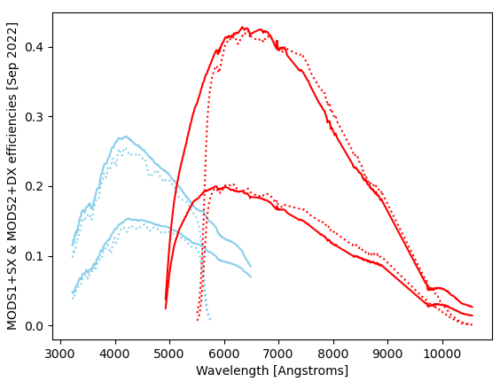
Figure 1: MODS1+SX and MODS2+DX airmass=0 efficiencies for direct (solid) and dual (dotted) grating modes from data taken in September 2022. The top pair of blue & red curves is for MODS2 and the bottom, for MODS1. All curves assume the same reflectivity (90%) for the primary and secondary mirrors, which may not be realistic, and so the value of the plot is mainly in illustrating the relative instrument+telescope throughput.
The spectroscopic zero points as a function of wavelength for the MODS1 grating modes, log Sλ ,0, are given in the table below.
The zeropoints in Table 1 (below) are from September 2022. The current sensitivity of MODS1+LBT-SX is about half that of MODS2+LBT-DX. Assuming this difference affects both the object and sky background similarly, for a given exposure time, the predicted signal-to-noise ratio of MODS1 would be about 1/sqrt(2) times that of MODS2 and, therefore, to achieve the same SNR with MODS1 as with MODS2 would require twice the exposure time.
Table1: MODS1+LBT-SX and MODS2+LBT-DX Grating Mode Spectroscopic Zero Points
The zeropoints in Table 1 are based on data taken in September and October 2022. The table was updated on 04-Nov-2022.
| MODS1 Red Grating | MODS2 Red grating | MODS1 Blue Grating | MODS2 Blue grating | ||||||
|---|---|---|---|---|---|---|---|---|---|
| λ(Å) | Direct logSλ,0 |
Dichroic log Sλ ,0 |
Direct logSλ,0 |
Dichroic log Sλ ,0 |
λ(Å) | Direct logSλ,0 |
Dichroic log Sλ ,0 |
Direct logSλ,0 |
Dichroic log Sλ ,0 |
| 5000 | 15.501 | … | 15.865 | … | 3200 | 15.091 | 15.016 | 15.485 | 15.431 |
| 5500 | 15.910 | 14.420 | 16.319 | 15.013 | 3500 | 15.388 | 15.349 | 15.766 | 15.746 |
| 6000 | 15.995 | 15.985 | 16.465 | 16.458 | 4000 | 15.728 | 15.681 | 16.026 | 15.992 |
| 6500 | 16.001 | 16.011 | 16.511 | 16.516 | 4500 | 15.814 | 15.788 | 16.070 | 16.059 |
| 7000 | 15.993 | 16.005 | 16.522 | 16.534 | 5000 | 15.819 | 15.809 | 16.045 | 16.044 |
| 7500 | 15.970 | 16.009 | 16.505 | 16.542 | 5500 | 15.797 | 15.763 | 15.991 | 15.955 |
| 8000 | 15.902 | 15.958 | 16.432 | 16.477 | 5800 | 15.764 | 14.459 | 15.956 | 14.597 |
| 8500 | 15.843 | 15.897 | 16.350 | 16.386 | 6000 | 15.719 | … | 15.902 | … |
| 9000 | 15.753 | 15.816 | 16.232 | 16.268 | 6450 | 15.622 | … | 15.799 | … |
| 9500 | 15.521 | 15.570 | 15.965 | 16.008 | |||||
| 10000 | 15.420 | 15.208 | 15.793 | 15.571 | |||||
Figures 2.1, 2.2 and 2.3, below, plot the sensitivity limits as a function of time for a given signal-to-noise ratio. These are based on measurements made with MODS1 and MODS2 in September & October 2022.
Figure 2.1: SNR tracks for MODS1 & MODS2 at g and r: For signal-to-noise ratios, SNR= 5, 20 and 100 per 0.5 (blue) or 0.85 angstrom (red) pixel in a spectrum that has been extracted over the number of rows corresponding to the seeing FWHM, tracks of AB magnitude vs time are plotted for both blue (at g_sdss/4770 angstroms) and red (r_sdss/6300 angstroms) channels. These tracks use the MODS1 and MODS2 dual grating zeropoints tabulated here and have been calculated for a 1″ slit, seeing FWHM = 1″, airmass = 1 and dark (new moon, solid lines) and bright (10-d moon, dotted lines) skies. The blue and red shaded regions indicate the range of magnitudes predicted for sky brightnesses from new to 10-d moon. The slit loss calculation assumes a Gaussian PSF, so for a slit width equal to the seeing FWHM, 24 percent of the light is lost. For the sky contribution, the area is the number of pixels covered by the slit width times the FWHM. The dark(bright) sky brightnesses at g_sdss and r_sdss were assumed to be 22.3(20.7) and 21.3(20.6), respectively. These are interpolated from the KPNO sky brightnesses and agree well with published dark sky values for Mt. Graham (Taylor+2004,PASP,116,762 and Pedani 2009, PASP,121,778).
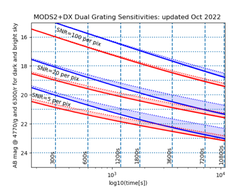
To do a “bye-eye interpolation” from this plot, recall that the SNR scales with the square root of the flux and of the exposure time, although for fainter objects whose flux is comparable to the sky brightness, SNR grows more slowly.
Caveat: The predicted SNRs should be considered best-case scenarios, as there are various observational factors that can degrade the actual SNR you see in your data: transparency, slit loss, sky brightness which can change with time (in the red, for example) and with telescope pointing (looking at a low elevation target in the direction of a city, e.g.). Also the predictions are based on photon statistics and do not account for uncertainties introduced in the data processing (e.g. flat-fielding errors). At the red end of the optical, especially at z, where the sky is brighter that at r and the CCD quantum efficiency is dropping, the predicted SNRs will be worse.
 |
 |
Figure 2.2 The same as in Figure 2.1, but the red channel predictions are made at i (7500 angstroms) instead of at r. At i, the sky brightnesses have been assumed to be 20.7 mag/sq.arcsec (dark) and 20.2 mag/sq.arcsec (bright). Click on the image to view it at full scale.
 |
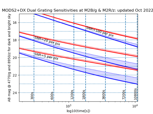 |
Figure 2.3 The same as in Figure 2.1, but the red channel predictions are made at z (8950 angstroms) instead of at r. At z, the sky brightnesses have been assumed to be 19.0 mag/sq.arcsec (dark) and 18.7 mag/sq.arcsec (bright).
Prism Mode
The efficiency curves, exclusive of the atmosphere, for dual and direct prism modes are shown below (These are for the MODS1 commissioning data from 2011, and as for the grating and imaging modes, we can expect a decline in the sensitivity of MODS1+SX). These curves will be updated.
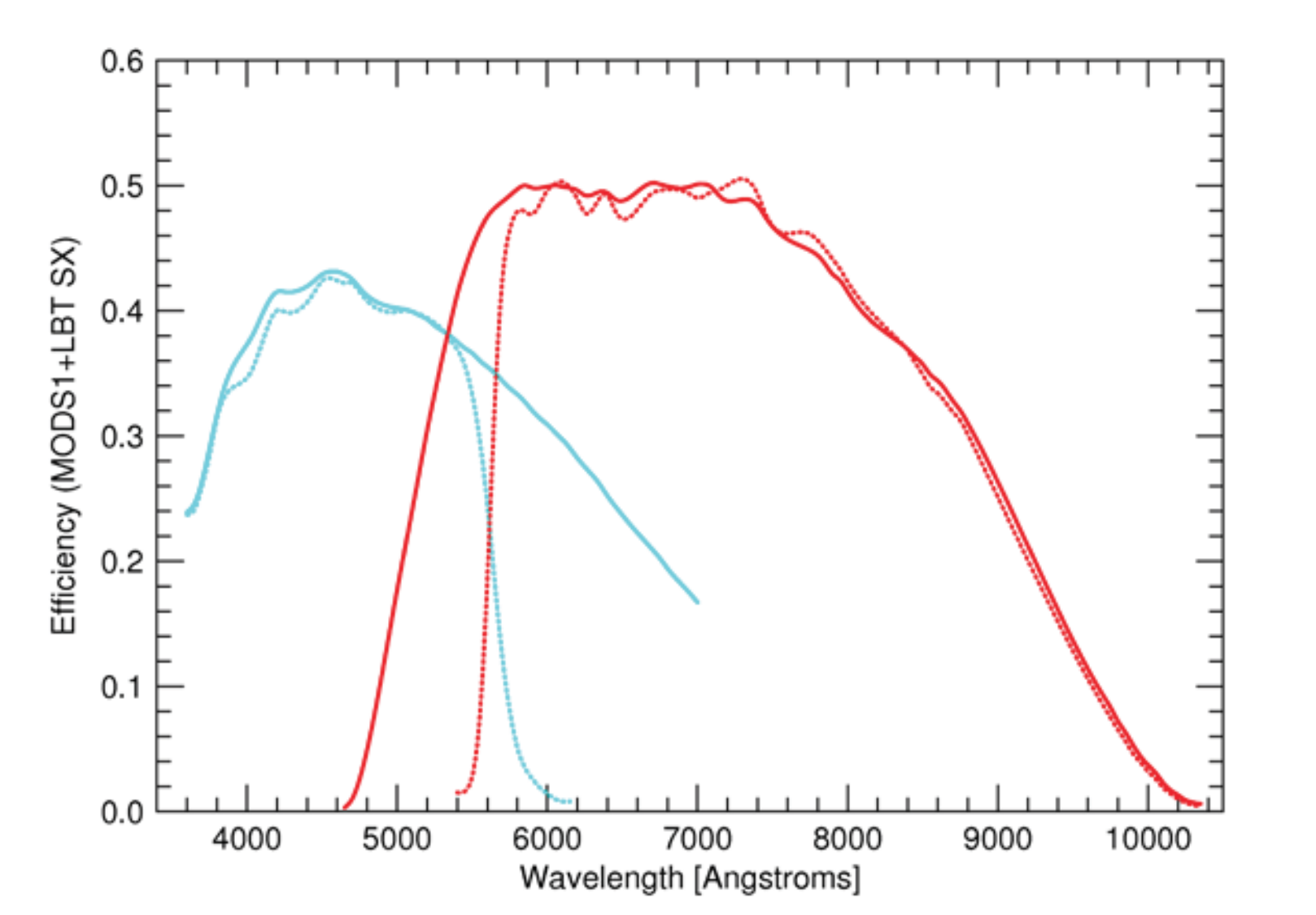 Figure 3: MODS1+LBT SX airmass=0 efficiencies for direct and dual prism modes (from the 2011 MODS1 Commissioning data). |
Spectroscopic zero points as a function of wavelength for the MODS1 prism modes are tabulated below:
Table 2: MODS1 Prism Mode Spectroscopic Zero Points
(based on MODS1 commissioning data taken in 2011)
| Red Prism | Blue Prism | ||||||
|---|---|---|---|---|---|---|---|
| log Sλ ,0 | Pixel | log Sλ ,0 | Pixel | ||||
| λ (Å) | Direct | Dichroic | δ λ (Å) | λ (Å) | Direct | Dichroic | δ λ (Å) |
| 5000 | 15.722 | … | 2.6 | 3600 | 15.663 | 15.640 | 3.4 |
| 5500 | 16.178 | 14.978 | 3.4 | 3850 | 15.886 | 15.858 | 4.4 |
| 6000 | 16.268 | 16.265 | 4.6 | 4030 | 15.978 | 15.927 | 5.1 |
| 6450 | 16.301 | 16.293 | 5.9 | 4500 | 16.121 | 16.096 | 7.1 |
| 7000 | 16.357 | 16.348 | 7.6 | 5000 | 16.162 | 16.138 | 9.8 |
| 7450 | 16.365 | 16.368 | 9.1 | 5500 | 16.172 | 16.112 | 12.7 |
| 8000 | 16.342 | 16.350 | 11.2 | 6000 | 16.143 | 15.478 | 15.8 |
| 8500 | 16.307 | 16.297 | 13.3 | 6450 | 16.082 | … | 18.5 |
| 8800 | 16.264 | 16.252 | 14.6 | 7000 | 15.964 | … | 21.8 |
| 9750 | 15.740 | 15.692 | 18.9 | ||||
| 10000 | 15.396 | 15.333 | 20.1 | ||||
The same formula for estimating counts per exposure time used for the grating mode apply to data in this table for the prism, but bear in mind that the size of spectral pixel is a strongly varying function of wavelength. Nominal pixel sizes are given in the final column for each side.
 |
Figure 3: For signal-to-noise ratios, SNR= 5, 20 and 100 per pixel in a prism spectrum that has been extracted over the number of rows corresponding to the seeing FWHM, tracks of AB magnitude vs time are plotted for both blue (at g_sdss/4770 angstroms) and red (r_sdss/6300 angstroms) channels. These tracks use the MODS1 dual prism zeropoints tabulated here and have been calculated for a 1″ slit, seeing FWHM = 1″, airmass = 1 and dark (new moon, solid lines) and bright (10-d moon, dotted lines) skies. With the prisms, the number of angstroms per pixel increases with wavelength, from ~3 angstroms/pix to ~20 angstroms/pix (see Table 2 above), so while the zeropoints for the prism and grating are similar, the predicted SNR per pixel is greater for the prism than for the grating, all other input parameters being equal. The blue and red shaded regions indicate the range of magnitudes predicted for sky brightnesses from new to 10-d moon. The slit loss calculation assumes a Gaussian PSF, so for a slit width equal to the seeing FWHM, 24 percent of the light is lost. For the sky contribution, the area is the number of pixels covered by the slit width times the FWHM. The dark(bright) sky brightnesses at g_sdss and r_sdss were assumed to be 22.3(20.7) and 21.3(20.6), respectively. These are interpolated from the KPNO sky brightnesses and agree well with published dark sky values for Mt. Graham (Taylor+2004,PASP,116,762 and Pedani 2009, PASP,121,778).
To do a “bye-eye interpolation” from this plot, recall that the SNR scales with the square root of the flux and of the exposure time, although for fainter objects whose flux is comparable to the sky brightness, SNR grows more slowly. Caveat: The predicted SNRs should be considered best-case scenarios, as there are various observational factors that can degrade the actual SNR you see in your data: transparency, slit loss, sky brightness which can change with time (in the red, for example) and with telescope pointing (looking at a low elevation target in the direction of a city, e.g.). Also the predictions are based on photon statistics and do not account for uncertainties introduced in the data processing (e.g. flat-fielding errors). At the red end of the optical, especially at z, where the sky is brighter that at r and the CCD quantum efficiency is dropping, the predicted SNRs will be worse.
Imaging Mode
Estimates of the imaging sensitivity of MODS are based on measurements of secondary photometric standard stars in the SDSS AB magnitude system (Clem, VandenBerg, and Stetson (2008)), and for those fields not covered by Clem et al, measurements of stars in the SDSS DR12 catalog. By manipulation of the photometric conversion formula,
mf = mf,0 – 2.5 log Sf + 2.5 log texp – Kf X
the predicted integrated counts in ADU in a filter given its SDSS AB magnitude in the filter band is given by:
log Sf = log Sf,0 – 0.4mf + log texp – 0.4 K f X
where:
log Sf = log counts in ADU for filter f
log Sf,0 = ADU zero point (counts for mf=0.0mag in 1 second) listed in the table below. [log Sf,0 = 0.4 mf,0]
mf = SDSS magnitude in filter f in AB units
mf,0 = photometric zero point magnitude in filter f in AB units listed in the table below.
texp = exposure time in seconds
Kf = estimated extinction coefficient for filter f
X = airmass at the time of the observation
Table 3: MODS ugriz Photometry ADU Zero Points and Zero Point Magnitudes
The zeropoints in Table 3 were measured from images of 4 fields with SDSS DR12 coverage that were observed on 2023 Feb 10 UT. These agree well with results based on data taken on 2021 Oct 27 UT. The largest discrepancies are for MODS1 u and MODS2 r (dual and direct, where the later results are 0.1 mag better). All of these data use the extinction coefficients measured during commissioning, which are given in the last column. The zeropoint and error was taken to be the median of the 4 or 5 images per configuration, and the number in parenthesis represents the spread. The spread is, in most cases, smaller than the standard deviation for an image, but when it is large, as at u, it cannot be explained by residual extinction and is probably is real scatter in the very small set of stars that were detected in some fields.
| Filter | MODS1 | MODS1 | MODS2 | MODS2 | Kf (mag/airmass) |
|---|---|---|---|---|---|
| mf,0 (mag) direct |
mf,0 (mag) dual |
mf,0 (mag) direct |
mf,0 (mag) dual |
||
| SDSS u | 24.80±0.13 (0.37) | 24.71±0.15 (0.26) | 26.11±0.05 (0.11) | 26.04±0.06 (0.08) | 0.47 |
| SDSS g | 26.81±0.06 (0.02) | 26.75±0.06 (0.03) | 27.46±0.06 (0.02) | 27.39±0.04 (0.04) | 0.17 |
| SDSS r | 26.41±0.09 (0.06) | 26.35±0.15 (0.06) | 27.82±0.03 (0.05) | 27.69±0.06 (0.06) | 0.10 |
| SDSS i | 26.29±0.10 (0.03) | 26.36±0.15 (0.08) | 27.63±0.03 (0.02) | 27.60±0.04 (0.07) | 0.05 |
| SDSS z | 25.67±0.10 (0.07) | 25.67±0.10 (0.08) | 27.10±0.05 (0.06) | 27.04±0.04 (0.15) | 0.03 |
The table below is based on MODS1 commissioning data taken in 2011, and these are the zeropoints used by the Imaging ETC.
| Filter | mf,0 (mag) | Kf | log Sf,0 |
|---|---|---|---|
| SDSS u | 25.68±0.12 | 0.47 | 10.25 |
| SDSS g | 27.38±0.03 | 0.17 | 10.94 |
| SDSS r | 27.24±0.03 | 0.10 | 10.90 |
| SDSS i | 27.21±0.04 | 0.05 | 10.91 |
| SDSSz | 26.41±0.04 | 0.03 | 10.58 |
A good rule of thumb is:
The peak pixel will saturate on an r = 15th mag in 30 sec in 0.6 arcsec seeing.
Model LBT Atmospheric Extinction
Table 4: LBT Model Extinction Curve
| λ (Å) | Kλ |
| 3200 | 0.866 |
| 3500 | 0.511 |
| 4000 | 0.311 |
| 4500 | 0.207 |
| 5000 | 0.153 |
| 5500 | 0.128 |
| 6000 | 0.113 |
| 6450 | 0.088 |
| 6500 | 0.085 |
| 7000 | 0.063 |
| 7500 | 0.053 |
| 8000 | 0.044 |
| 8210 | 0.043 |
| 8260 | 0.042 |
| 8370 | 0.041 |
| 8708 | 0.026 |
| 10256 | 0.020 |
The coefficients in this model LBT extinction curve do not include strong telluric absorption features, so this correction should be done with caution if using it to predict signal in a given exposure time at wavelengths in proximity to strong telluric features.