MODS ETC — calculations
This page provides the equations and assumptions used by the MODS ETC.
The Signal-to-Noise Ratio
The signal-to-noise is given by the ratio:
(1) 
where the C![]() is the number of electrons from the object, C
is the number of electrons from the object, C![]() , the number of electrons from the sky, RN is the readnoise (e
, the number of electrons from the sky, RN is the readnoise (e![]() /pix) and N
/pix) and N![]() is the number of pixels over which the signal is integrated. We assume that object and sky noise obey Poisson statistics. The RN for each of the MODS detectors is given on the Detector Characteristics page. The dark current is negligible, 0.4-0.5 e-/s/hr. Other sources of noise: e.g. elevated backgrounds from stray light or well overflow; vary from image to image and are not considered here.
is the number of pixels over which the signal is integrated. We assume that object and sky noise obey Poisson statistics. The RN for each of the MODS detectors is given on the Detector Characteristics page. The dark current is negligible, 0.4-0.5 e-/s/hr. Other sources of noise: e.g. elevated backgrounds from stray light or well overflow; vary from image to image and are not considered here.
The spectroscopic (log S![]() ) and imaging (m
) and imaging (m![]() ) zeropoints enable the prediction of the number of counts per angstrom, S
) zeropoints enable the prediction of the number of counts per angstrom, S![]() [ADU/
[ADU/![]() ], from a source of given flux density, F
], from a source of given flux density, F![]() [erg/s/cm
[erg/s/cm![]() ] at wavelength
] at wavelength ![]() , when observed at an airmass, X, and with exposure time, t
, when observed at an airmass, X, and with exposure time, t![]() . The extinction coefficient, K
. The extinction coefficient, K![]() [mag/airmass] for the LBT model atmosphere is assumed.
[mag/airmass] for the LBT model atmosphere is assumed.
(2) ![]()
In the case of imaging, where the input flux is usually given as a magnitude, i.e. m![]() at filter
at filter ![]() , and the zeropoints are also given as magnitudes, m
, and the zeropoints are also given as magnitudes, m![]() , the predicted number of counts in the bandpass,
, the predicted number of counts in the bandpass, ![]() , log
, log ![]() [ADU], can be expressed as:
[ADU], can be expressed as:
(3) ![]()
where the following relation between m![]() and log
and log ![]() is used:
is used:
(4) ![]()
where ![]() , the pivot wavelength of the band:
, the pivot wavelength of the band: ![]() .
.
For extended sources as well as for the sky background, where the input magnitude or flux density is per square arcsecond, the formulas below predict counts per angstrom per square arcsecond [ADU/![]() /square arcsecond] (spectroscopy) or counts per square arcsecond within the bandpass
/square arcsecond] (spectroscopy) or counts per square arcsecond within the bandpass ![]() [ADU/square arcsecond] (imaging).
[ADU/square arcsecond] (imaging).
To convert from ![]() or
or ![]() (for obj or sky) to C
(for obj or sky) to C![]() or C
or C![]() requires the conversion gain, g [ADU/electrons], and some assumptions about the extraction parameters and the shape of the PSF, for point sources. In the following, the pixel size,
requires the conversion gain, g [ADU/electrons], and some assumptions about the extraction parameters and the shape of the PSF, for point sources. In the following, the pixel size, ![]() = 0.12″/pix for the blue camera and 0.123″/pix for the red.
= 0.12″/pix for the blue camera and 0.123″/pix for the red.
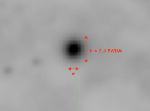
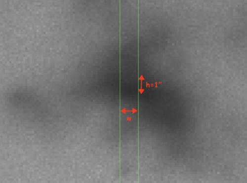
These assumptions are described below and depicted in figure at the bottom of this page for point (left) and extended source (right) spectroscopy:
Spectroscopic
The SNR per pixel uses the following formulae where ![]() is the slit width and
is the slit width and ![]() the height of the extraction window in pixels. The linear dispersion,
the height of the extraction window in pixels. The linear dispersion, ![]() [
[![]() /pixel] is used to convert from electrons per angstrom to electrons per pixel.
/pixel] is used to convert from electrons per angstrom to electrons per pixel.
(5) ![]()
(6) ![]()
Point Source
For point source spectroscopy, a Gaussian PSF is assumed in both calculating the fraction of light entering the slit, ![]() , and in determining the height of the extraction window,
, and in determining the height of the extraction window, ![]() .
.
(7) 
The height of the extraction window, ![]() , is taken to be
, is taken to be ![]() FWHM since for a Gaussian PSF that will admit 99.5% of the object’s light:
FWHM since for a Gaussian PSF that will admit 99.5% of the object’s light:
(8) ![]()
The number of pixels over which the spectrum is integrated for the SNR estimate is:
(9) ![]()
To predict whether the spectrum at wavelength ![]() will be saturated, the
will be saturated, the ![]() is again assumed to have a Gaussian profile and this is integrated spatially over the just central pixel and divided by the gain:
is again assumed to have a Gaussian profile and this is integrated spatially over the just central pixel and divided by the gain:
(10) ![]()
The counts in the peak pixel, ![]() , are then the sum of counts from object, sky
, are then the sum of counts from object, sky ![]() and bias
and bias ![]() . The ETC assumes a coarse average,
. The ETC assumes a coarse average, ![]() ADU.
ADU.
(11) 
Extended Source
For extended source spectroscopy, the total counts from the source are the product of the surface brightness and the area of slit width ![]() the extraction window, which in this case does not depend on the seeing and is chosen to be 1″. In equations (5) and (6) above:
the extraction window, which in this case does not depend on the seeing and is chosen to be 1″. In equations (5) and (6) above:
![]() and
and ![]() arcsec.
arcsec.
In this case,
(12) ![]()
Counts in the peak pixel are:
(13) 
Imaging
(14) ![]()
and
(15) ![]()
In the above, ![]() is the fraction of light in the software aperture of diameter,
is the fraction of light in the software aperture of diameter, ![]() , and
, and ![]() represents the area [sq arcseconds] of the aperture.
represents the area [sq arcseconds] of the aperture.
The number of pixels in that aperture, ![]() .
.
Point Source
For point source imaging, the total counts from the source are integrated over the software aperture. We (somewhat arbitrarily) assume an aperture with diameter ![]() , which for a Gaussian PSF would contain 93.6% of the object’s light.
, which for a Gaussian PSF would contain 93.6% of the object’s light.
(16) ![]()
The software aperture has an area, ![]() square arcseconds and covers
square arcseconds and covers ![]() pixels.
pixels.
The Gaussian PSF is integrated over the peak pixel and added to sky and bias contributions to estimate the counts in the peak pixel as:
(17) 
Extended Source
For extended source imaging, the total counts from the object and from the sky are calculated both within a square region of area 1″ x 1″:
![]() and
and ![]() ; and within a single pixel:
; and within a single pixel: ![]() and
and ![]() .
.
We assume that no light is lost within the chosen aperture, i.e. ![]()
Counts in the peak pixel are estimated to be:
(18) 
 |
 |

